

All intelligent life on Earth learns through association. From the moment a baby recognizes a face, to a bird realizing that a rustle in the grass may mean food, intelligence is built on patterns. We associate cause with effect, input with outcome, experience with expectation, and this forms the core of the learning process. Associative learning is a fundamental process where two events become linked in memory, creating a new response. Machine learning works in much the same way. Instead of the nerves and emotions, computers rely on numbers and algorithms, but the essence remains the same: learning from patterns in data. These models are designed to uncover associations and use them to make predictions. Some of them learn by asking simple yes or no questions, some by drawing lines through data, and others by mimicking the layered reasoning of the human brain.
The simplest way a computer can “think” is through a yes or no split, called a decision stump. Linking many of these together forms a decision tree. Each branch of the tree represents a question about the data, eventually leading to an output at a leaf. In real-world datasets, there are often many features, and not all of them line up neatly with a single tree. To decide which question to ask next, trees use measures such as entropy, which reflects how random the data is, error rate, which measures inaccuracy, and mutual information, which captures how much knowing one feature helps predict another. In this way, decision trees grow by reducing confusion, minimizing mistakes, and asking the most informative questions first.
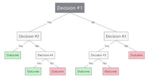
A decision tree
Source: https://blog.mindmanager.com/wp-content/uploads/2022/03/Decision-Tree-Diagram-Example-MindManager-Blog.png
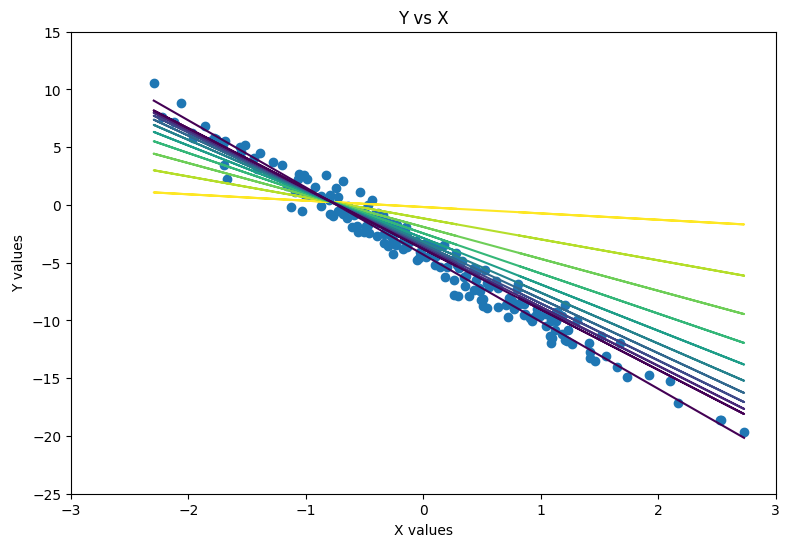
Sometimes, the best way to understand a relationship is to draw a straight line through it. That is the idea behind linear regression. It is a model that tries to capture how one variable may affect another variable. It allows the user to use multiple continuous variables to predict a target value with high precision. There are multiple ways to train a linear regression model. One possible way is using gradient descent. This method starts with an initial guess for the model’s parameters and repeatedly adjusts them to minimize the loss, which is the inaccuracy of the model. At each step, we calculate the gradient, which tells us how to change the parameters to reduce the error. By moving in the direction that decreases the loss, the model gradually improves its predictions. For very large datasets, stochastic gradient descent is often used, which updates the model using one data point or a small batch at a time to make learning faster. Polynomial regression extends linear regression by allowing the model to fit curved relationships. It does this by adding higher-degree terms like x2, x3, and so on, which lets the line bend to capture more complex patterns. This increases the risk of overfitting though, especially with high-degree polynomials, so it’s important to balance complexity with generalization.

Evolution of the ‘line of best fit’
Sometimes we just want a yes or no probability distribution. This is where logistic regression comes in. Logistic regression handles these cases by transforming the linear combination of features through a nonlinear activation function, often the sigmoid curve, which compresses any input into a probability between zero and one. So, logistic regression builds on the ideas of linear regression but adapts them for classification tasks. The process starts by looking at the input features, such as grades or attendance, and combining them using the model weights. This scales up the features differently, meaning features having more influence on the output get a higher weight. The activation function then transforms this score into a probability. There are different activation functions to choose from, like the Sigmoid, Tanh, ELU, and ReLU, and each one of them has their own uses. Training the model involves adjusting the weights to make better predictions. Again, gradient descent can be used for training. The trained model weights can be used to predict new outcomes and see the probability of the predicted outcome.
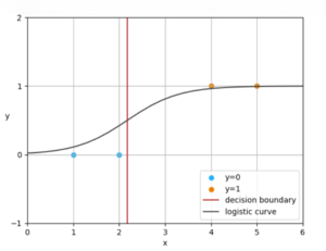
Logistic regression decision boundary and the sigmoid curve
Logistic regression is powerful for binary decisions, but what if the data is too complex for a single curve to capture? That is where we use neural networks, models which mimic the layered thinking of the brain. At their core, these are just stacks of logistic regression models, which are present as neurons in the hidden and the output layers. Ideally, according to the Universal Approximation Theorem, all functions can be plotted with a 1-hidden layer neural network with a 0% error, given there exists an enough number of neurons, and the right activation functions. In a typical 3-layer network, the input layer takes in the input values, scales them up differently by the corresponding weights, and then applies a non-linear activation function to the weighted inputs to get to the hidden layer neurons. These neurons are then scaled up by their weights, and passed through a softmax function, which returns the probability distribution of all the classes. This is called forward propagation, through which we can calculate the loss of the neural network function. We can also calculate the gradient of the network by using the chain rule to find the derivative of the neural network’s overall function. This is known as backward propagation. Both forward and backward propagation can be used to train the model using the gradient descent algorithm. The trained model weights can then be used for predictions. A commonly used subset of neural networks is the convolutional neural network (CNN). CNN layers use filters that slide across the data, learning to detect local features such as edges, textures, and shapes. These features are then combined into increasingly complex patterns across deeper layers, which makes CNNs especially effective at tasks like image classification and facial recognition.
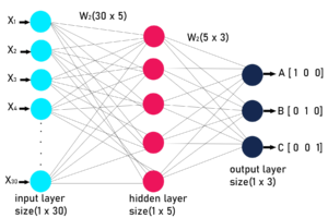
Architecture of a 3-layer neural network
Source: https://media.geeksforgeeks.org/wp-content/uploads/20200522110034/NURELNETWORK.jpg
In essence, facial recognition models, which are built on convolutional neural networks, which are a subset of neural networks, which are hierarchies of logistic regression models, which are an extension of linear regression, recognize faces through the simple act of drawing lines through data.
Leave a Reply